Discover more from Capital Flows

Capital Flows is the space where I share all my Top-Down/Bottom-up macroeconomic research and show how I am tangibly implementing it in financial markets.

Over 5,000 subscribers

The Research Hub: Risk On / Risk Off Regimes

How do you know what regime you are in?

Capital Flows

Aug 23, 2023

Hey everyone,

There is a lot of discussion out there as to if we are still in a bear market or have entered a new bull market. What complicates things further is everyone seems to have a different definition of a bull or bear market that they assert is “the correct definition”, as if something could even be possible.

Do you know why financial advisors and media spokespeople use this? It’s because it’s a way to skirt the actual issue. It’s pure marketing and misdirection. I hear people say the “official definition” of exiting a bear market is some artificial number or some type of “inflation-adjusted return.”

If I ever tried to play semantic shenanigans to justify losses or lack of proper attribution analysis for financial assets, I’d be fired immediately. Just imagine a PM walking into his boss’s office after losing money and saying to his boss, “I don’t know sir, technically I haven’t officially lost money if we adjust it for inflation.”

When we think about moves in asset markets, we want to quantify with specificity so that we can have a greater ability to confirm or falsify a view we might hold. This is where we get into quantifying market regimes. The way in which you quantify market regimes is directly connected to the type of timeframe and risk tolerance you have. For example, if you want to avoid drawdowns but miss out on some upside potential, you might implement a vol control strategy in your portfolio that reduces exposure incrementally as specific signals are triggered. If you want a book on this idea, check out Strategic Risk Management.

This is why when people ask, are we in a bull market or bear market, anyone who is actually managing risk is going to say, well, what’s your timeframe and risk preference?

In this article we will go through some examples, go through regime identification and then how to actually quantify regimes correctly.

Simple Regimes:

A lot of people use moving averages or Bollinger Bands to define if we are in a bull or bear market. This is totally fine! There are obviously much better ways to quantify regimes though. Going through examples and interpreting signal-to-noise is how you begin to understand the limitation and benefits of quantitive signals.

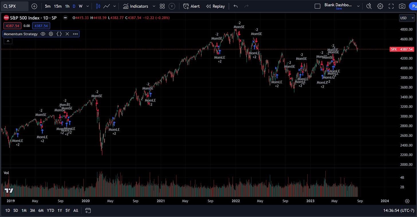
In the first example, let’s say we use a simple moving average to go long or short:

Notice that the simple moving average helps you catch a lot of the major trends but a lot of times there is noise and false signals. Now remember the logic of a moving average, it is trying to smooth returns. There is nothing wrong with this as long as you understand the limitations of smoothing returns.

If you used a pure rolling returns strategy that doesn’t smooth the time series then you will get more signals:

A lot of times people will try blending these signals to make decisions or scale position sizes.

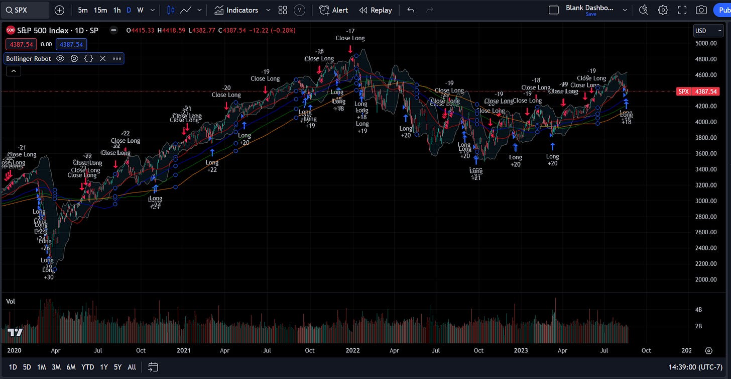
The other popular way people might define regimes is through standard deviation or Bollinger bands:

For both the moving average strategy and Bollinger bands, you can change the look back or stdv which changes the frequency at which signals are generated. This frequency at which signals are generated is connected to your goals.

Now you can see, if you simply change the look back or inputs of a model, the frequency and quality of its signals can change. This will connect to how you want to manage your portfolio. Even when someone provides their “official definition”, that is likely biased to a specific situation and hasn’t been backtested, their definition is simply a different set of inputs that has different statistical validity.

The best thing you can do when these marketing phrases and “official definitions” are thrown at you is to ask questions.

Is there a better way to quantify market regimes than the simple moving averages and Bollinger Bands? Yes, but it is still shocking how few people implement it.

Let’s dig into it!

Markov Models:

Markov Models or Markov Type Model Logic is how I approach quantifying market regimes.

What is a Markov Model? Here is a technical definition:

A Markov Model is a statistical model used to represent systems that transition from one state to another according to certain probabilistic rules. The defining characteristic of a Markov Model is the Markov property, which states that the probability of transitioning to any particular state depends solely on the current state and time elapsed, and not on the sequence of states that preceded it.

Markov Models are widely used in various fields such as physics, chemistry, economics, and particularly in computer science for algorithms in machine learning, natural language processing, and data compression, among others. The model can be represented as a set of states, transitions between these states, and the probabilities associated with these transitions.

There are several types of Markov Models, including:

Discrete-time Markov Chains: The state transitions occur at discrete time steps.
Continuous-time Markov Chains: The state transitions occur continuously over time.
Hidden Markov Models: The state is not directly visible, but the output, dependent on the state, is visible.
Markov Decision Processes: An extension of Markov Chains that include decisions, rewards, and objectives.

Each type has its own specific use-cases and methods for analysis and prediction.

Resources:

There are a ton of resources on Markov Models because they can be built with multiple different inputs.

Here are some papers to start with:

https://www.twosigma.com/wp-content/uploads/2021/10/Machine-Learning-Approach-to-Regime-Modeling_.pdf

https://papers.ssrn.com/sol3/papers.cfm?abstract_id=1714016

https://papers.ssrn.com/sol3/papers.cfm?abstract_id=2845809

https://papers.ssrn.com/sol3/papers.cfm?abstract_id=1138782

https://papers.ssrn.com/sol3/papers.cfm?abstract_id=49240

https://papers.ssrn.com/sol3/papers.cfm?abstract_id=3406068

https://papers.ssrn.com/sol3/papers.cfm?abstract_id=2472768

https://papers.ssrn.com/sol3/papers.cfm?abstract_id=3759243

https://papers.ssrn.com/sol3/papers.cfm?abstract_id=2557236 (this is a good one)

https://papers.ssrn.com/sol3/papers.cfm?abstract_id=4217513

https://papers.ssrn.com/sol3/papers.cfm?abstract_id=532122

https://papers.ssrn.com/sol3/papers.cfm?abstract_id=1081337

Makes Intuitive Sense:

If you feel like the whole Markov Model is a bit too complicated, just think about it like this. In a world of complexity, there are never clear signals. You want to use “fuzzy logic” in order to frame situations. Think about it like this, there is never a single definition, signal, or rule for when you should say “I love you” to the person you started dating. You gotta read the room because every circumstance is different. It makes intuitive sense that complex situations with many false signals require a different type of thinking.

Let’s go through a very specific example of a Markov model so that we can make all of this a bit more tangible: https://papers.ssrn.com/sol3/papers.cfm?abstract_id=3144169

I really like this paper because it is super simplistic but has a lot of good principles for expanding into more complex quantification of Markov Models:

The main idea of this paper is we are defining states of a time series differently and then stacking those functions to see where these different states overlap to indicate a specific probable outcome:

Notice how the functions stack on top of each other to create a regime that has higher specificity. Then you can define them into different quadrants. Great regime specificiation allows you to be more intentional about your actions.

Then you can run multiple assets through it and run your correlation analysis on the actual regimes instead of the raw time series:

This idea of correlations is what brings us to my final thought of “risk on/risk off regimes.”

Give a gift subscription

Risk On/Risk Off:

We have gone over the idea of regimes purely based on the time series. However, if we want to begin adding more “fundamental” metrics and correlations to further specify regimes into risk on/risk off (RORO) regimes, we can do this by quantifying risk premiums across all major assets.

I wrote a 5 part FX Primer that went into a lot of detail about risk premiums:

5-Part FX Primer Breakdown:

Basically, if we begin quantifying how risk premiums function across assets then correlations begin making more sense as we move through various growth, inflation, and liquidity regimes.

This is how we begin to define RORO regimes because they are marked by a pervasive expansion or contraction in risk premiums. If you begin to match a risk premia matrix with a correlation matrix and then your Markov Model, you will have a lot more visibility into the current environment.

Conclusion:

Everything will come down to how you quantify these dynamics and how you are able to match them to the specific constraints of a situation. A financial product is simply a quantified way of meeting the constraints of a specific situation.

The building blocks are literally all there. You just need to spend the time creating something that is exceptional.

Feel free to reach out any time with questions via Twitter DM or email.

In the information age, you simply need to be at the right place, at the right time, with the right information to succeed

Thanks for reading!

Give a gift subscription